Step 2. Identifying interesting behaviour

To investigate the changes happening between samples, we need to define which samples represent which conditions and the subjects from which the samples were taken. This allows us to directly compare protein expression in different conditions, analysing the samples in those conditions as a whole.

The way that we do this depends on both the origin of our samples and how they were treated. This is because that information will determine the correct statistical treatment. The Experiment Design Setup screen offers 2 options:

• Between Subject: samples from any given subject appear in only one condition e.g. control subjects versus subjects with different drug treatments.
• Within Subject: here, samples have been taken from a given subject under different conditions e.g. the same subject has been sampled over a period of time, or after one or more treatments.

This tutorial experiment's design—control samples vs. treated—matches the first of these two, so:

1. Click anywhere within the Between Subject option.
2. In the window that appears, enter Control vs. Treated in the Name field.
3. Click the Create Design button.

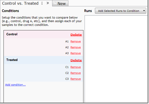
We now need to group our control and treated samples:

1. Click on each of the following runs to highlight them: A1, A2 and A3.
2. Click the Add Selected Runs to Condition button. A new condition, named Condition 1, will appear in the list at the left.
3. Click on the new condition's name to edit it; enter the name Control.
4. Repeat the above 3 steps for the remaining runs, naming the second condition Treated.

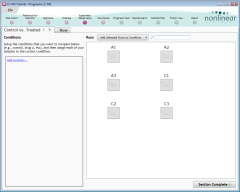
Your experiment design should now look like this. Click Section Complete to continue.

Finding statistically significant differences

The View Results screen is a powerful, and visually rich, screen that helps you to:

• Find features that show interesting variation between conditions
• Mark—or ‘tag’—and filter those features
• Review and, where needed, edit the results of feature detection

For simplicity, we'll skip the review and editing of detected features, and we'll concentrate on finding the interesting features. For this experiment, we want to identify features whose abundance is signficantly greater in the treated samples compared to the control samples.

We'll start by finding features whose abundance changes significantly either way:

1. Right-click on any feature in the list at the left of the screen.
2. From the pop-up menu that appears, select the Anova p-value ≤ 0.05 option in the Quick Tags sub-menu.
3. When the Create New Tag window appears, enter the name Significant change and click OK.

All features that have an Anova (p) value of less than or equal to 0.05 will now have a red tag in the list's Tag column.

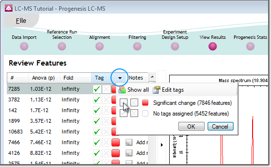
Tagging features, as we have done here, is the primary way of creating a list of peptides that require further attention. However, we also need to filter the list of features based on the tags we create:

1. Click the small arrow in the title of the Tag column. This will display the tag filter pop-up.
2. Click on the tick alongside the Signficant change tag.
3. Click OK to apply the filter. This updates the list to show only the features that have the Signficant change tag.

Finding specific expression behaviours

Using this list, we can now apply further filtering criteria. In our case, we want to find features that are more abundant in our treated group:

1. Click the Section Complete button to progress to the Progenesis Stats screen.
2. As the screen loads, it will begin calculating a Principal Components Analysis (“PCA”) plot of our filtered features. Click the Cancel Calculation button on the progress indicator to save a bit of time; for this tutorial, we don't need a PCA plot.
3. Click on the Ask Another Question button near the top-left of the screen.
4. From the menu that appears, select the second entry: Correlation Analysis. The software will then start its calculations.

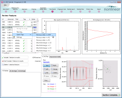
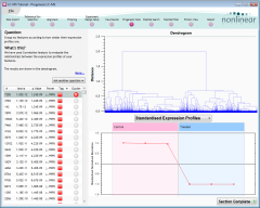
Once complete, the upper half of the Progenesis Stats screen shows a dendrogram. By clicking on its branching points, we can view the expression profiles of all features under that branch. Try exploring this yourself – it's an interesting way to learn about your data. When you're satisfied, click the right-hand branch at the top branching level, as shown here:

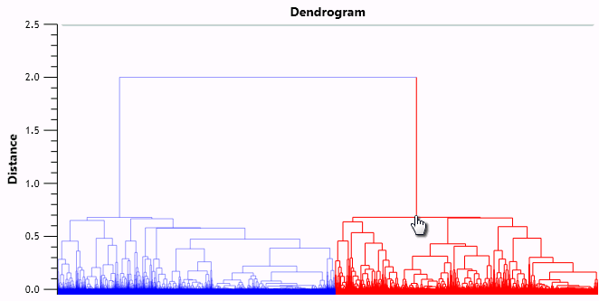
As you will see in the expression profiles below the dendrogram, this branch contains features that are more abundant in our Treated samples than in the Control samples. We'll keep track of these features by creating another tag:

1. Click the small arrow in the title of the Tag column to display the tag filter pop-up.
2. In the pop-up, click the Edit Tags... button.
3. In the Edit Tags window, click the Create New Tag button, enter a tag name of Up in Treated and click OK.
4. Click OK in the Edit Tags window to confirm the new tag.

All of the features in the selected dendrogram branch will now have the Up in Treated tag. We have now achieved our aim of identifying features whose abundance is signficantly greater in the treated samples compared to the control samples.

Of course, there are many more ways to explore your data in the View Results and Progenesis Stats screens. It's a good idea to read more about this after you finish this tutorial.

For the moment, however, click the Section Complete button to move to the Peptide Search screen, where we'll begin identifying the peptides…